Chapter 5 Shape Constrained-Generalized Additive Models
In order to fit SDM in agreement with the ecological niche theory, the proposed Shape-Constrained Generalized Additive Models (SC-GAMs) in (Citores et al. 2020) are fitted in this section. SC-GAMs are based on Generalized Additive Models, allowing us to impose shape-constraints to the linear predictor function. The R package SCAM implements the general framework developed by (Pya and Wood 2015) using shape-constrained P-splines. Monotonicity and concavity/convexity constraints can be imposed on the sign of the first and/or the second derivatives of the smooth terms. For fitting Species Distribution Models in agreement with the ecological niche theory, we imposed concavity constraints (\(f''(x) \le 0\)), so that the response can presents at most a single mode.
Alternatively, the R package mboost fits SC-GAMs using boosting methods. We are not going to develop this alternative here.
First, we load the list of required libraries.
requiredPackages <- c("here", "rstudioapi",
    "stringr", "RColorBrewer", "ggplot2",
    "dplyr", "fields", "maps", "raster",
    "scam", "plotmo", "pkgbuild", "dismo")
We run a function to install the required packages that are not in our system and load all the required packages.
install_load_function <- function(pkg) {
    new.pkg <- pkg[!(pkg %in% installed.packages()[,
        "Package"])]
    if (length(new.pkg))
        install.packages(new.pkg, dependencies = TRUE)
    sapply(pkg, require, character.only = TRUE)
}

install_load_function(requiredPackages)
## here rstudioapi stringr RColorBrewer ggplot2 dplyr
## TRUE TRUE TRUE TRUE TRUE TRUE
## fields maps raster scam plotmo pkgbuild
## TRUE TRUE TRUE TRUE TRUE TRUE
## dismo
## TRUEWe define some overall settings.
# General settings for ggplot
# (black-white background, larger
# base_size)
theme_set(theme_bw(base_size = 16))
5.1 Model fit
We set the working directory to the folder where the current script is located and we load the dataset (PAdata_with_env.Rdata) containing the presence-absence data together with the environmental data.
To fit a logistic regression model in the SC-GAMs framework, we use the scam function, where we set the binomial family with the logit link function. Our response variable is the presence-absence data and the selected three explanatory variables are the SST, chlorophyll and salinity. Each variable is included in the model through an spline function where the concavity constraint is set using bs=“cv”. The details about this option can be found in the section “Constructor for concave P-splines in SCAMs” of the SCAM manual (https://cran.r-project.org/web/packages/scam/scam.pdf). The number of knots (k) is fixed at 8 in this example for a good balance between flexibility and computation time.
UNIVARIATE MODELS
Before fitting the model with the selected three environmental variables, we can fit univariate model as follows.
We fit the univariate model for SST, we print the summary of the model fit, and look at the fitted curve in the response scale.
model_sst <- scam(occurrenceStatus ~ s(BO_sstmean,
    k = 8, bs = "cv"), family = binomial(link = "logit"),
    data = data)
summary(model_sst)
##
## Family: binomial
## Link function: logit
##
## Formula:
## occurrenceStatus ~ s(BO_sstmean, k = 8, bs = "cv")
##
## Parametric coefficients:
## Estimate Std. Error z value Pr(>|z|)
## (Intercept) -2.24702 0.08182 -27.46 <2e-16 ***
## ---
## Signif. codes: 0 '***' 0.001 '**' 0.01 '*' 0.05 '.' 0.1 ' ' 1
##
## Approximate significance of smooth terms:
## edf Ref.df Chi.sq p-value
## s(BO_sstmean) 2 2 1078 <2e-16 ***
## ---
## Signif. codes: 0 '***' 0.001 '**' 0.01 '*' 0.05 '.' 0.1 ' ' 1
##
## R-sq.(adj) = 0.2607 Deviance explained = 23.1%
## UBRE score = 0.066363 Scale est. = 1 n = 29661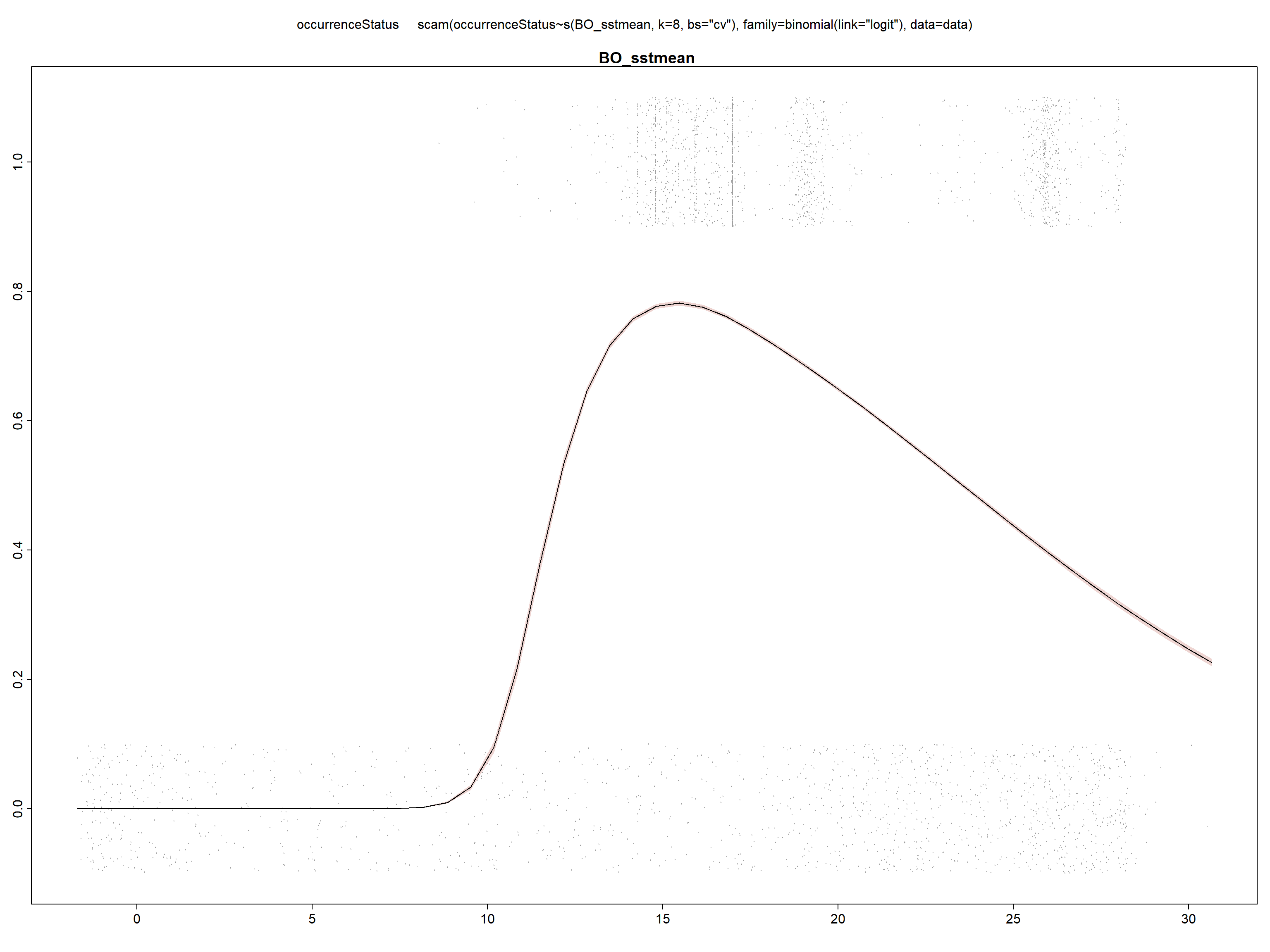
We repeat the same steps for the rest of the variables.
model_chl <- scam(occurrenceStatus ~ s(BO2_chlomean_ss,
    k = 8, bs = "cv"), family = binomial(link = "logit"),
    data = data)
summary(model_chl)
##
## Family: binomial
## Link function: logit
##
## Formula:
## occurrenceStatus ~ s(BO2_chlomean_ss, k = 8, bs = "cv")
##
## Parametric coefficients:
## Estimate Std. Error z value Pr(>|z|)
## (Intercept) 0.12663 0.01333 9.499 <2e-16 ***
## ---
## Signif. codes: 0 '***' 0.001 '**' 0.01 '*' 0.05 '.' 0.1 ' ' 1
##
## Approximate significance of smooth terms:
## edf Ref.df Chi.sq p-value
## s(BO2_chlomean_ss) 1 1 3263 <2e-16 ***
## ---
## Signif. codes: 0 '***' 0.001 '**' 0.01 '*' 0.05 '.' 0.1 ' ' 1
##
## R-sq.(adj) = 0.1546 Deviance explained = 12.4%
## UBRE score = 0.21423 Scale est. = 1 n = 29661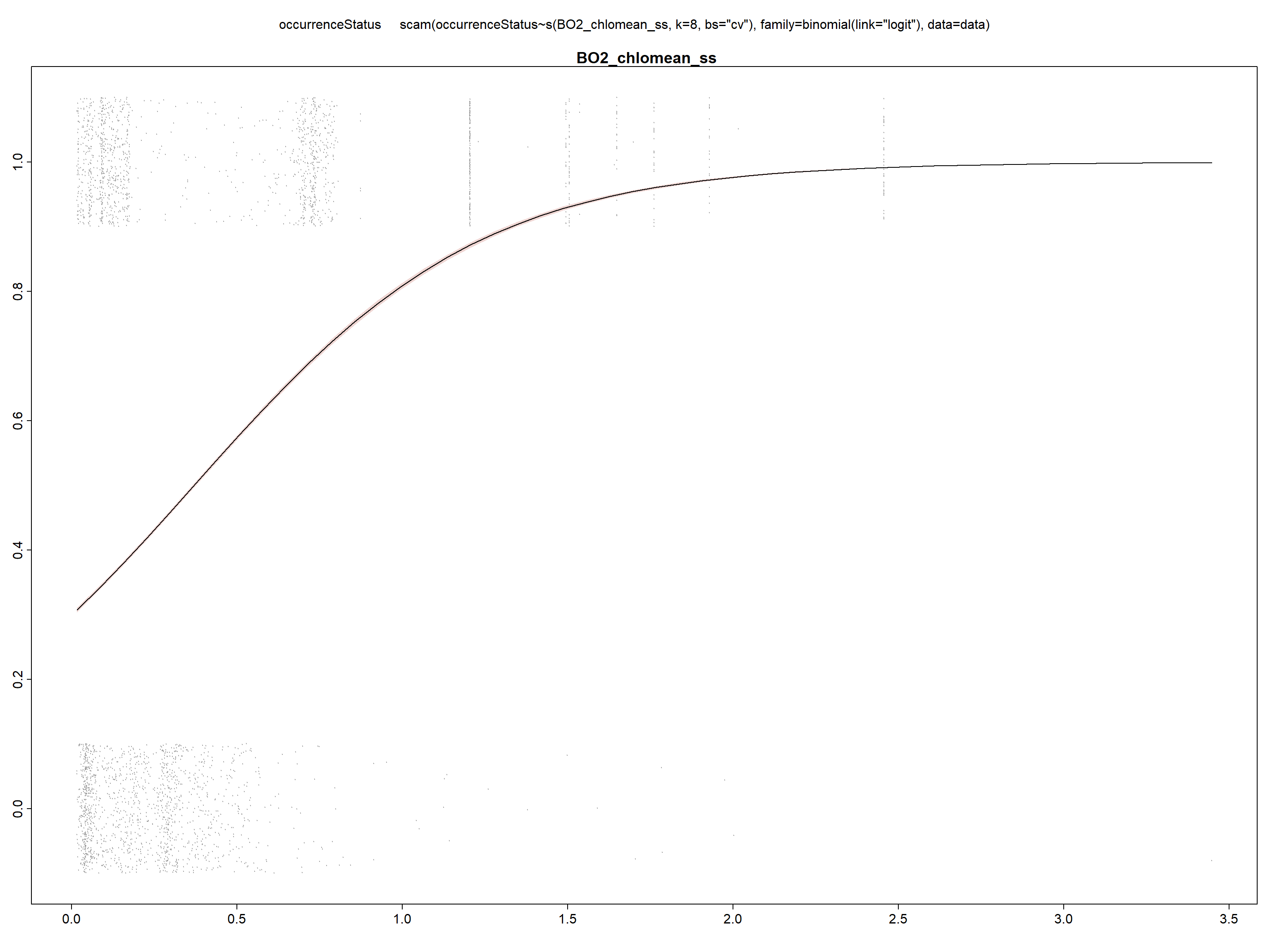
Due to convergence issues, sometimes it is necessary to fix the smoothing parameter (sp) at small value, i.e. \(10^{-5}\), as here when introducing salinity as an explanatory variable. If no value is provided, the smoothing parameter is estimated within the model.
model_sal <- scam(occurrenceStatus ~ s(BO2_salinitymean_ss,
    k = 8, bs = "cv"), family = binomial(link = "logit"),
    data = data, sp = 1e-05)
summary(model_sal)
##
## Family: binomial
## Link function: logit
##
## Formula:
## occurrenceStatus ~ s(BO2_salinitymean_ss, k = 8, bs = "cv")
##
## Parametric coefficients:
## Estimate Std. Error z value Pr(>|z|)
## (Intercept) -0.1445 0.0138 -10.47 <2e-16 ***
## ---
## Signif. codes: 0 '***' 0.001 '**' 0.01 '*' 0.05 '.' 0.1 ' ' 1
##
## Approximate significance of smooth terms:
## edf Ref.df Chi.sq p-value
## s(BO2_salinitymean_ss) 2 2 893.8 <2e-16 ***
## ---
## Signif. codes: 0 '***' 0.001 '**' 0.01 '*' 0.05 '.' 0.1 ' ' 1
##
## R-sq.(adj) = 0.0514 Deviance explained = 4.38%
## Scale est. = 1 n = 29661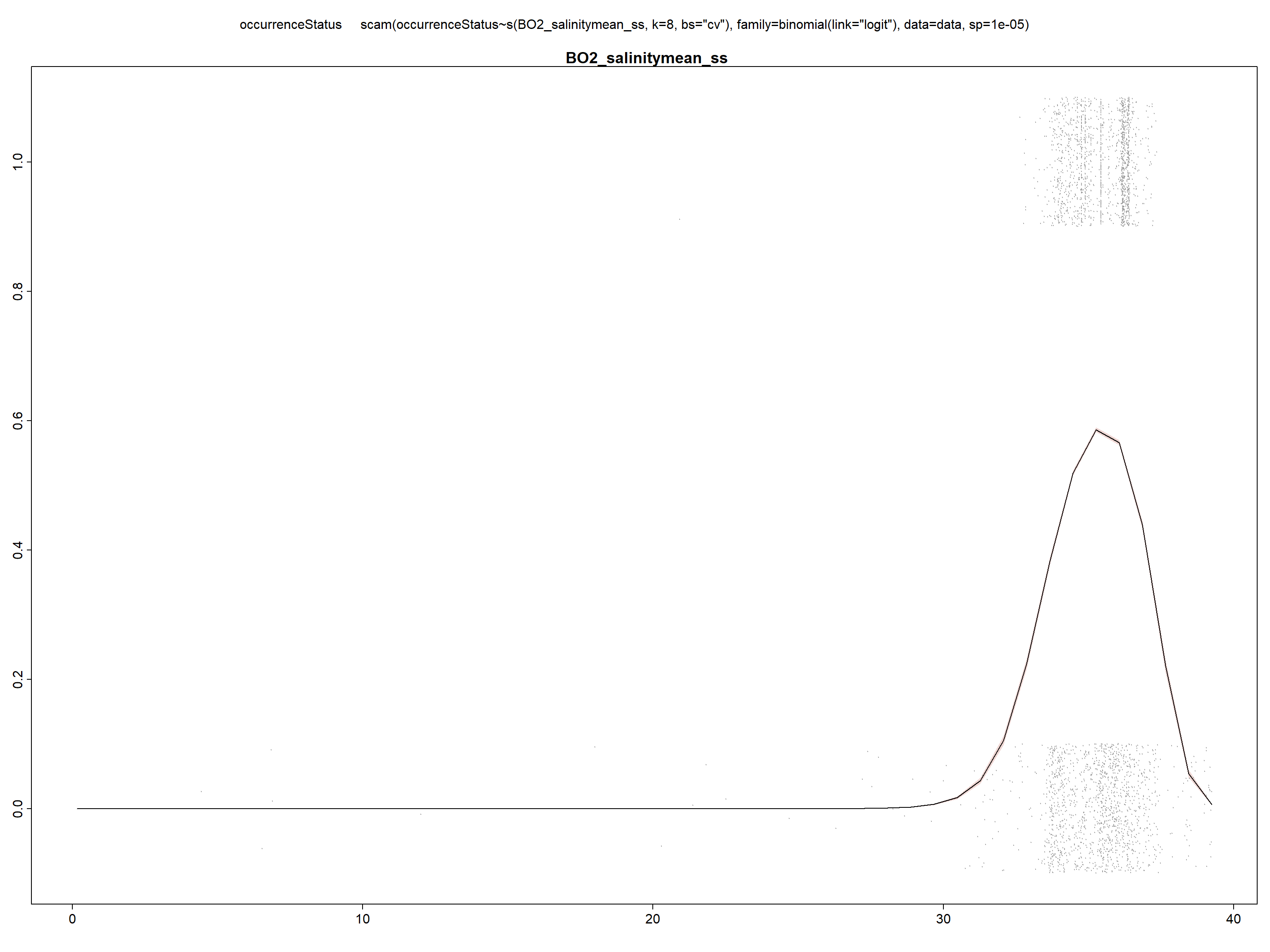
MODEL WITH ALL VARIABLES
Now we fit the model including the three selected variables.
model <- scam(occurrenceStatus ~ s(BO_sstmean,
    k = 8, bs = "cv") + s(BO2_salinitymean_ss,
    k = 8, bs = "cv") + s(BO2_chlomean_ss,
    k = 8, bs = "cv"), family = binomial(link = "logit"),
    data = data, sp = rep(1e-05, 3))
summary(model)
##
## Family: binomial
## Link function: logit
##
## Formula:
## occurrenceStatus ~ s(BO_sstmean, k = 8, bs = "cv") + s(BO2_salinitymean_ss,
## k = 8, bs = "cv") + s(BO2_chlomean_ss, k = 8, bs = "cv")
##
## Parametric coefficients:
## Estimate Std. Error z value Pr(>|z|)
## (Intercept) -1.813 3.163 -0.573 0.567
##
## Approximate significance of smooth terms:
## edf Ref.df Chi.sq p-value
## s(BO_sstmean) 4.001 4.003 765.8 <2e-16 ***
## s(BO2_salinitymean_ss) 2.004 2.008 178.7 <2e-16 ***
## s(BO2_chlomean_ss) 3.987 4.003 1778.0 <2e-16 ***
## ---
## Signif. codes: 0 '***' 0.001 '**' 0.01 '*' 0.05 '.' 0.1 ' ' 1
##
## R-sq.(adj) = 0.3491 Deviance explained = 32%
## Scale est. = 1 n = 29661## plotmo grid: BO_sstmean BO2_salinitymean_ss BO2_chlomean_ss
## 18.89921 35.42666 0.2452632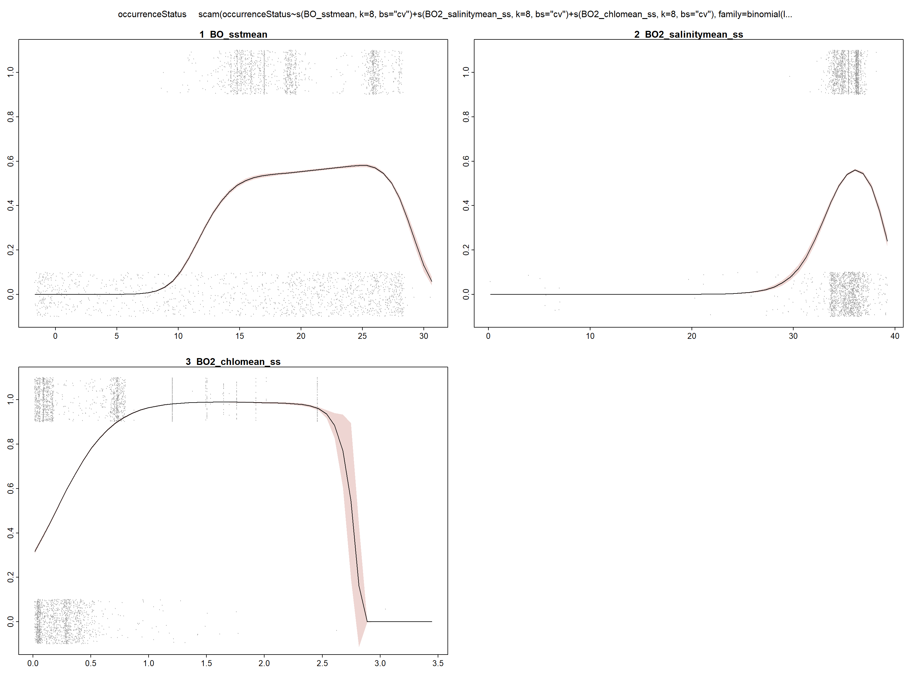
We can see in the summary of the fit, that all included variables are statistically significant (with p<0.05) and present a unimodal response curve.
For a more detailed check of the fitting, we can use the scam.check function:
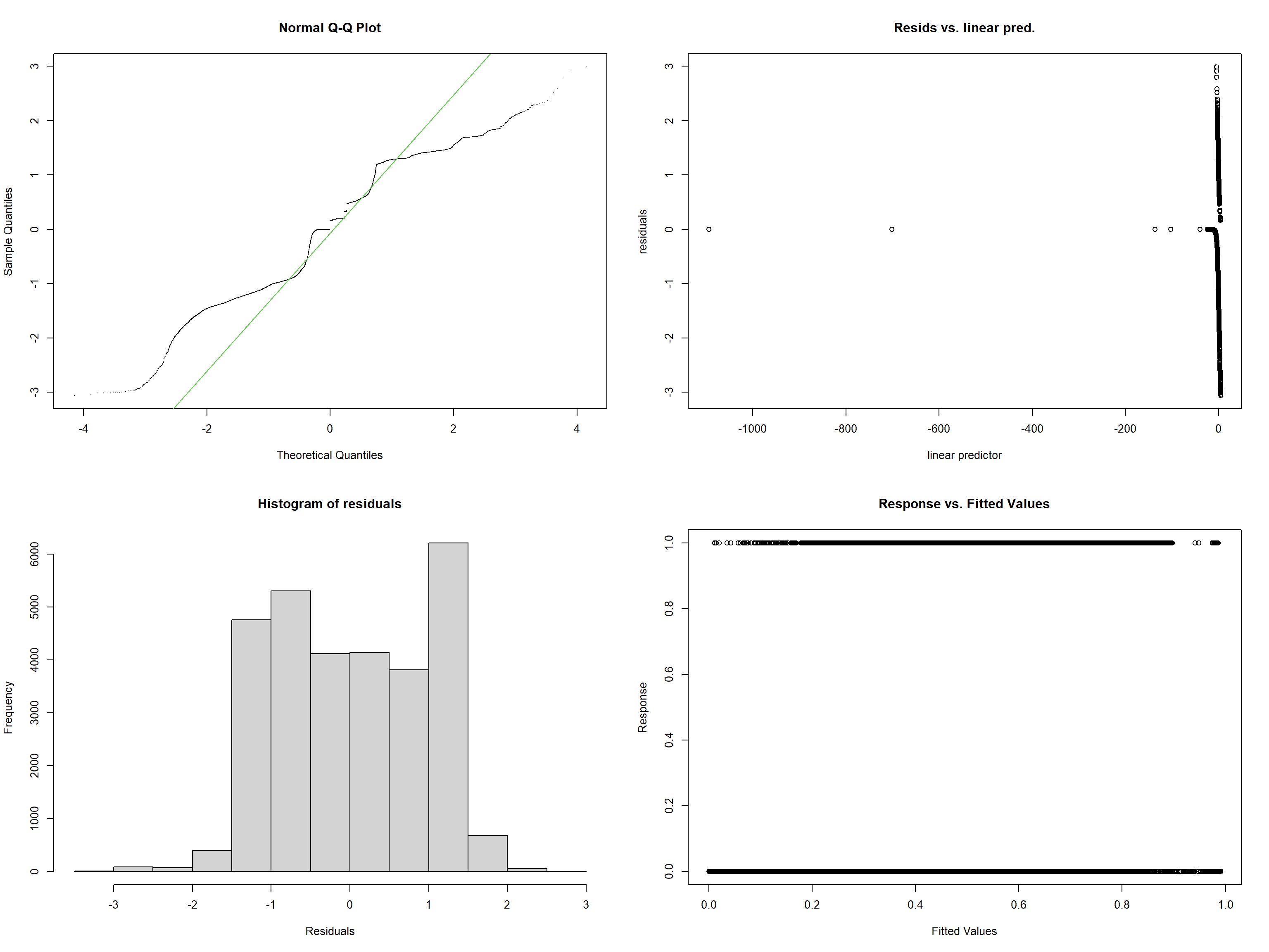
##
## Method: UBRE   Optimizer: NA newton
## The optimal smoothing parameter(s): 1e-05 1e-05 1e-05 .
5.2 Model selection
When several explanatory variables are available, a variable selection process can be carried out. Here we provide as an example, a function that performs forward variable selection (modsel.scam) based on the significance of variables and AIC values of the fits.
We save the names of the variables we want to introduce for the variable selection process as a vector:
The default AIC tolerance is 2 and there is not a limit on selected terms in this example. These options can be modified through aic.tol and vmax arguments in the function. The number of knots and the sp can be also modified.
model_SCGAM <- try(modsel.scam(basef = "occurrenceStatus ~ 1",
    vars = vars, dat = data, sp = 1e-05),
    silent = T)
## [1] "Fitting models with 1 terms"
## occurrenceStatus ~ 1+s(BO_sstmean,m=2,bs='cv',k=8)
## occurrenceStatus ~ 1+s(BO2_salinitymean_ss,m=2,bs='cv',k=8)
## occurrenceStatus ~ 1+s(BO2_chlomean_ss,m=2,bs='cv',k=8)
## [1] "Fitting models with 2 terms"
## occurrenceStatus ~ 1+s(BO_sstmean,m=2,bs='cv',k=8)+s(BO2_salinitymean_ss,m=2,bs='cv',k=8)
## occurrenceStatus ~ 1+s(BO_sstmean,m=2,bs='cv',k=8)+s(BO2_chlomean_ss,m=2,bs='cv',k=8)
## [1] "Fitting models with 3 terms"
## occurrenceStatus ~ 1+s(BO_sstmean,m=2,bs='cv',k=8)+s(BO2_chlomean_ss,m=2,bs='cv',k=8)+s(BO2_salinitymean_ss,m=2,bs='cv',k=8)We check results of the selected model, such as, selected variable names:
## [1] "BO_sstmean" "BO2_chlomean_ss" "BO2_salinitymean_ss"AICs of the fitted models:
##                null          BO_sstmean     BO2_chlomean_ss BO2_salinitymean_ss
##            41120.17            31629.40            28318.30            27990.07
Explained deviance of fitted models:
##                null          BO_sstmean     BO2_chlomean_ss BO2_salinitymean_ss
##       -1.769524e-16        2.309141e-01        3.117433e-01        3.198121e-01
Formulas of the fitted models:
## $null
## occurrenceStatus ~ 1
##
## $BO_sstmean
## occurrenceStatus ~ 1 + s(BO_sstmean, m = 2, bs = "cv", k = 8)
## <environment: 0x0000021e7c51a510>
##
## $BO2_chlomean_ss
## occurrenceStatus ~ 1 + s(BO_sstmean, m = 2, bs = "cv", k = 8) +
##     s(BO2_chlomean_ss, m = 2, bs = "cv", k = 8)
## <environment: 0x0000021e7c51a510>
##
## $BO2_salinitymean_ss
## occurrenceStatus ~ 1 + s(BO_sstmean, m = 2, bs = "cv", k = 8) +
##     s(BO2_chlomean_ss, m = 2, bs = "cv", k = 8) + s(BO2_salinitymean_ss,
##     m = 2, bs = "cv", k = 8)
## <environment: 0x0000021e7c51a510>
Summaries of the fitted models:
## $null
##
## Family: binomial
## Link function: logit
##
## Formula:
## occurrenceStatus ~ 1
##
## Parametric coefficients:
##             Estimate Std. Error z value Pr(>|z|)
## (Intercept) 0.009777   0.011613   0.842      0.4
##
##
## R-sq.(adj) =      0   Deviance explained = -1.77e-14%
## UBRE = 0.38634  Scale est. = 1         n = 29661
##
## $BO_sstmean
##
## Family: binomial
## Link function: logit
##
## Formula:
## occurrenceStatus ~ 1 + s(BO_sstmean, m = 2, bs = "cv", k = 8)
## <environment: 0x0000021e7c51a510>
##
## Parametric coefficients:
##             Estimate Std. Error z value Pr(>|z|)
## (Intercept) -2.24678    0.08094  -27.76   <2e-16 ***
## ---
## Signif. codes:  0 '***' 0.001 '**' 0.01 '*' 0.05 '.' 0.1 ' ' 1
##
## Approximate significance of smooth terms:
##               edf Ref.df Chi.sq p-value
## s(BO_sstmean)   2      2   1082  <2e-16 ***
## ---
## Signif. codes:  0 '***' 0.001 '**' 0.01 '*' 0.05 '.' 0.1 ' ' 1
##
## R-sq.(adj) =  0.2607   Deviance explained = 23.1%
##   Scale est. = 1         n = 29661
##
##
## $BO2_chlomean_ss
##
## Family: binomial
## Link function: logit
##
## Formula:
## occurrenceStatus ~ 1 + s(BO_sstmean, m = 2, bs = "cv", k = 8) +
##     s(BO2_chlomean_ss, m = 2, bs = "cv", k = 8)
## <environment: 0x0000021e7c51a510>
##
## Parametric coefficients:
##             Estimate Std. Error z value Pr(>|z|)
## (Intercept)   -3.057      9.021  -0.339    0.735
##
## Approximate significance of smooth terms:
##                      edf Ref.df Chi.sq p-value
## s(BO_sstmean)      4.000  4.000  939.7  <2e-16 ***
## s(BO2_chlomean_ss) 4.221  3.952 2225.6  <2e-16 ***
## ---
## Signif. codes:  0 '***' 0.001 '**' 0.01 '*' 0.05 '.' 0.1 ' ' 1
##
## R-sq.(adj) =  0.341   Deviance explained = 31.2%
##   Scale est. = 1         n = 29661
##
##
## $BO2_salinitymean_ss
##
## Family: binomial
## Link function: logit
##
## Formula:
## occurrenceStatus ~ 1 + s(BO_sstmean, m = 2, bs = "cv", k = 8) +
##     s(BO2_chlomean_ss, m = 2, bs = "cv", k = 8) + s(BO2_salinitymean_ss,
##     m = 2, bs = "cv", k = 8)
## <environment: 0x0000021e7c51a510>
##
## Parametric coefficients:
##             Estimate Std. Error z value Pr(>|z|)
## (Intercept)   -1.813      3.163  -0.573    0.567
##
## Approximate significance of smooth terms:
##                          edf Ref.df Chi.sq p-value
## s(BO_sstmean)          4.001  4.003  765.8  <2e-16 ***
## s(BO2_chlomean_ss)     3.987  4.003 1778.1  <2e-16 ***
## s(BO2_salinitymean_ss) 2.004  2.008  178.7  <2e-16 ***
## ---
## Signif. codes:  0 '***' 0.001 '**' 0.01 '*' 0.05 '.' 0.1 ' ' 1
##
## R-sq.(adj) =  0.3491   Deviance explained =   32%
##   Scale est. = 1         n = 29661
The last model of the list, is the selected one. Which in this case contains the considered three variables.
We save the selected model
Note that there are multiple options and criteria for model selection that are not reviewed here. Any model selection technique used for GAMs can be used also for SC-GAMs.