Chapter 7 Prediction and maps
In this chapter we predict from the fitted model and produce final SDMs maps.
First, we load a list of required libraries.
requiredPackages <- c(
  "here",
  "rstudioapi",
  "ggplot2",
  "tidyverse",
  # "rgdal",
  "raster",
  "maps",
  "RColorBrewer",
  "scam",
  "ggpubr"
  )
We run a function to install the required packages that are not in our system and load all the required packages.
install_load_function <- function(pkg) {
    new.pkg <- pkg[!(pkg %in% installed.packages()[,
        "Package"])]
    if (length(new.pkg))
        install.packages(new.pkg, dependencies = TRUE)
    sapply(pkg, require, character.only = TRUE)
}

install_load_function(requiredPackages)
## here rstudioapi ggplot2 tidyverse raster maps
## TRUE TRUE TRUE TRUE TRUE TRUE
## RColorBrewer scam ggpubr
## TRUE TRUE TRUEWe define some overall settings.
# General settings for ggplot
# (black-white background, larger
# base_size)
theme_set(theme_bw(base_size = 16))
7.1 Prepare environmental data
In previous steps (see Chapter 2), we have defined the study area that defines the extent of our spatial data. We load the study_area object that is a SpatialPolygonsDataFrame class:
And we load the rasterStack with the downloaded environmental data.
We transform the environmental data set first into a data frame, and then into a SpatialDataFrame.
##        x                y            mylayers_1        mylayers_2
##  Min.   :-97.79   Min.   :-82.96   Min.   :0.0       Min.   : 0.1
##  1st Qu.:-56.23   1st Qu.:-39.73   1st Qu.:0.1       1st Qu.:33.8
##  Median :-14.67   Median :  3.50   Median :0.3       Median :34.6
##  Mean   :-14.67   Mean   :  3.50   Mean   :0.3       Mean   :34.4
##  3rd Qu.: 26.90   3rd Qu.: 46.73   3rd Qu.:0.4       3rd Qu.:35.6
##  Max.   : 68.46   Max.   : 89.96   Max.   :3.6       Max.   :40.7
##                                    NA's   :1501044   NA's   :1501044
##    mylayers_3        mylayers_4
##  Min.   :0.0       Min.   :-1.8
##  1st Qu.:0.0       1st Qu.: 1.9
##  Median :0.0       Median :15.1
##  Mean   :0.1       Mean   :13.7
##  3rd Qu.:0.1       3rd Qu.:24.1
##  Max.   :1.0       Max.   :32.3
## NA's :1652879 NA's :16528797.2 Projection
We load the selected model and predict into the whole environmental data.
# Load SC-GAM model
load(here::here("models", "selected_model.Rdata"))

# Predicting
predict <- predict(selected_model, newdata = env_dataframe,
    type = "response", se.fit = T)

env_dataframe$fit <- predict$fit
env_dataframe$se.fit <- predict$se.fit

save(env_dataframe, file = "results/projection.Rdata")
7.3 Mapping
# Load PA data
load(here::here ("data", "outputs_for_modelling", "PAdata_with_env.Rdata"))


proj_map <-ggplot()+
  geom_raster(data=subset(env_dataframe),
              aes(x,y,fill=fit)) +
  scale_fill_gradient2(low="blue",
                       mid="orange",
                       high="red",
                       midpoint = 0.5,
                       limits = c(0,1)) +
  ggtitle("Occurrence probabilty Thunnus alalunga")+
  geom_point(data=subset(data,occurrenceStatus==1),
             aes(LON,LAT),
             col=1,
             size=0.3) +
  theme_pubclean(base_size = 14)+
  theme(panel.background = element_blank(),
        plot.title = element_text(face = "italic"),
        #text = element_text(size = 14),
        axis.text.x = element_text(size = 10),
        axis.text.y = element_text(size = 10),
        legend.position="right") +
  labs(y="latitude", x = "longitude")

print(proj_map)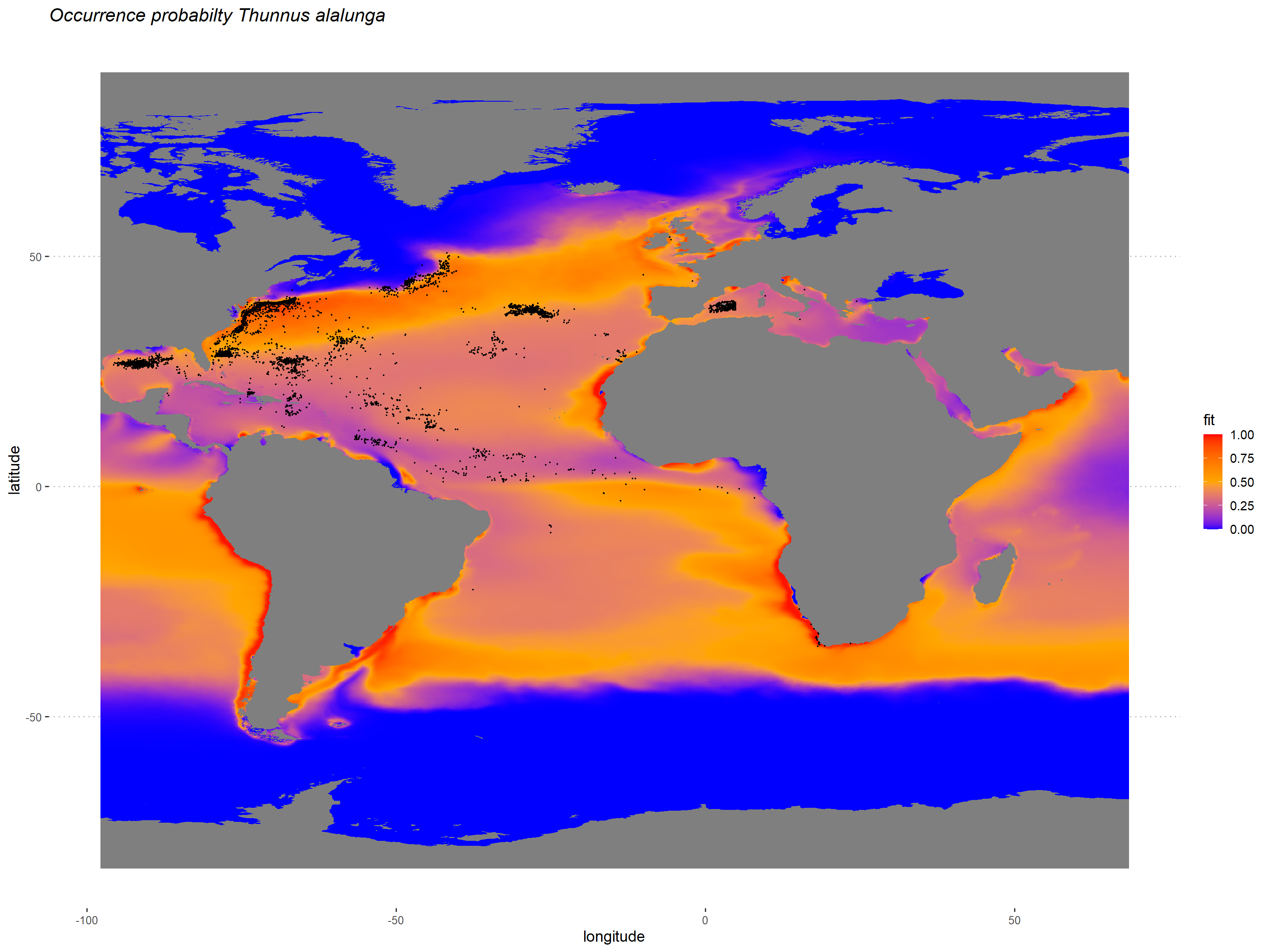
We finally save the projection map.