Chapter 5 Extract the information from the netCDF files
Once you have downloaded the oceanographic data, you will probably want to extract information for a set of observations. In this section, we present a simple way to do this extraction.
5.1 Read your observations
Let’s assume you have your observations saved as a CSV file. We are going to use this dataset as example. The first step is to read the CSV file:
require(readr)
my_data = read_delim("https://raw.githubusercontent.com/GiancarloMCorrea/extractOceanVariables/refs/heads/main/data/example_data.csv", delim=";")
head(my_data)
## # A tibble: 6 × 3
## Lon_M Lat_M Date
## <dbl> <dbl> <date>
## 1 -81.1 -3.45 2015-02-20
## 2 -81.6 -3.45 2015-02-20
## 3 -81.2 -3.45 2015-02-20
## 4 -81.6 -3.44 2015-02-20
## 5 -81.1 -3.45 2015-02-20
## 6 -81.8 -3.44 2015-02-20This dataset may have several columns, but it should have at least three columns with the following information: longitude (numeric), latitude (numeric), and date (character, %Y-%m-%d). There should not be missing information (i.e., NA) for these three columns.
5.2 Extract oceanographic data
To extract the oceanographic data, we will use the matchCOPERNICUS function (you can find it here). The instructions provided below work when downloading multiple .nc files as explained in Section 2.6.
matchCOPERNICUS creates a new column in your observations dataframe (i.e., my_data) with the oceanographic variable that corresponds to the longitude/latitude/date combination of every row.
Before extracting the oceanographic variable, we will load the matchCOPERNICUS, required libraries, and some auxiliary functions directly from Github:
source("https://raw.githubusercontent.com/GiancarloMCorrea/extractOceanVariables/refs/heads/main/code/copernicus/multiple/matchCOPERNICUS.R")
source("https://raw.githubusercontent.com/GiancarloMCorrea/extractOceanVariables/refs/heads/main/code/auxFunctions.R")
require(dplyr)
require(lubridate)
require(stars)
Then, we extract the data:
my_data = matchCOPERNICUS(
            data         = my_data,
            lonlat_cols  = c("Lon_M", "Lat_M"),
            date_col     = "Date",
            var_label    = "sst",
            var_path     = "C:/Use/env_data/",
            depth_FUN    = "mean",
            depth_range  = c(0, 25)
)datais the dataframe with the observations.lonlat_colsis a character vector with the column names of the longitude and latitude indata.date_colsis a character with the column name of the date indata.var_labelis the name of the column that will be created with the oceanographic data. It does not need to be the same as the variable name you are extracting.var_pathis the path where the.ncfiles are saved.
Since we are matching information using longitude/latitude/date, the depth dimension needs to be summarized somehow. depth_FUN is the function that will be applied to summarize all the information within the depth_range vector (in meters).
For monthly oceanographic data, matchCOPERNICUS will extract the information for the corresponding month.
matchCOPERNICUS has also another argument called nc_dimnames:
Which is a character vector with the longitude, latitude, and date dimension names in the .nc files. By default, it is set to c("x", "y", "time"), but you can change it if needed.
5.3 Plot the extracted oceanographic information
It is always important to plot the extracted environmental variable to check if the matching has been correctly done. First, let’s create a new column containing the month for every row:
Then, we could make a simple plot using the ggplot2 package:
require(sf)
require(viridis)
require(ggplot2)
# Find longitude and latitude ranges in our observations
xLim = range(my_data$Lon_M) + 0.5*c(-1, 1)
yLim = range(my_data$Lat_M) + 0.5*c(-1, 1)
# Transform our observations to sf point object:
MyPoints = my_data %>% st_as_sf(coords = c("Lon_M", "Lat_M"), crs = 4326, remove = FALSE)
# Get worldmap object:
worldmap = ggplot2::map_data("world")
colnames(worldmap) = c("X", "Y", "PID", "POS", "region", "subregion")
# Make plot:
ggplot() +
  geom_sf(data = MyPoints, aes(color = sst), size = 0.5) +
  scale_colour_viridis() +
  geom_polygon(data = worldmap, aes(X, Y, group=PID), fill = "gray60", color=NA) +
  coord_sf(expand = FALSE, xlim = xLim, ylim = yLim) +
  xlab(NULL) + ylab(NULL) +
  theme_classic() +
  facet_wrap(~ month)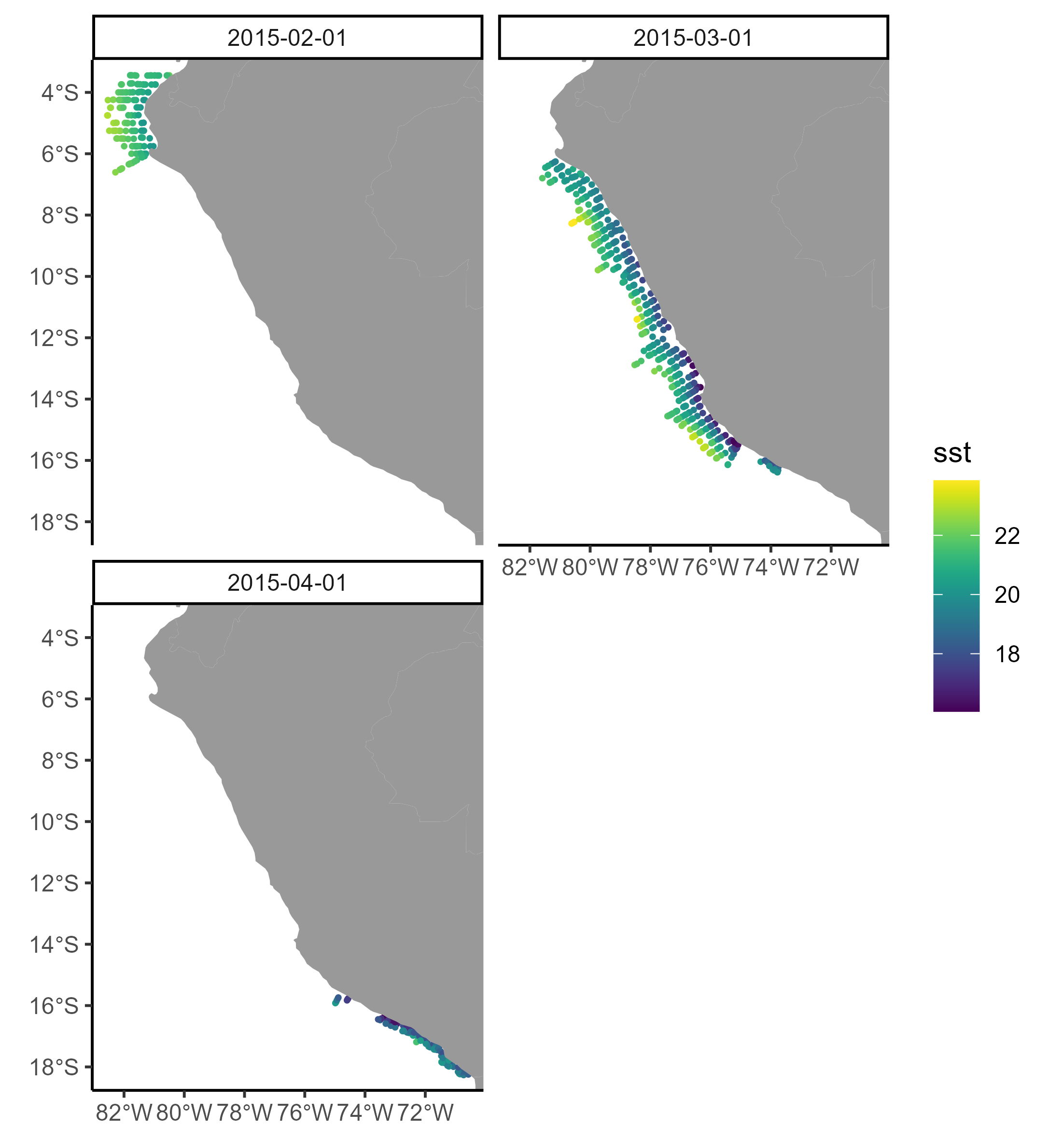
5.4 Imputation of missing information
In some cases, there may be NA when extracting the oceanographic data. We could fill these NA using the mean value around the location with missing information. We have made an R function, called fill_NAvals to do so (you can find it here and was loaded above).
my_data = fill_NAvals(
                data         = my_data,
                lonlat_cols  = c("Lon_M", "Lat_M"),
                var_col      = "sst",
                group_col    = "month",
                radius       = 10
)datais the dataframe with the observations.lonlat_colsis a character vector with the column names of the longitude and latitude indata.var_colis a character with the column name of the oceanographic variable indata.group_colis the name of the column that will be used as grouping. For example, we might only want to average month-specific locations when fillingNA.radiusdefines the radius (km) around the location with missing information to calculate the average.